Simulating data#
This guide describes how to use the simulation utilities provided by the library.
Currently, only LC-MS simulation is implemented. The aim of the simulation utilities is not to synthesize signals that mimic real world signals, but to provide tools that can be used to test and develop data pipelines. Despite this, the simulation utilities allow to take into account several effects observed on real datasets:
inter-sample variation in compounds abundance
compound prevalence
instrumental variation in spectra
time-dependent signal loss
inter-batch signal variation
signal from multiple isotopologues
Two tools are provided for this end:
SimulatedLCMSSampleFactory: A factory class that createsSamplemodels with synthesized data that behaves in the same way as a sample with real data.simulate_data_matrix(): a function that creates a data matrix with simulated data.
We’ll start by showing an example of how sample data can be created. Then, we will cover the
SimulatedLCMSAdductSpec which defines the properties of
features in simulated samples. Finally we will describe in detail sample and matrix data simulation.
Introductory example#
The following code block allows to create a simulated sample with three adducts:
from tidyms2.simulation.lcms import SimulatedLCMSSampleFactory
from tidyms2.io import MSData

adducts_spec = [
    {
        "formula": "[C54H104O6]+",
        "rt": {"mean": 10.0},
    },
    {
        "formula": "[C27H40O2]+",
        "rt": {"mean": 20.0},
    },
    {
        "formula": "[C24H26O12]+",
        "rt": {"mean": 30.0},
    },
]

simulated_sample_factory = SimulatedLCMSSampleFactory(adducts=adducts_spec)
sample = simulated_sample_factory(id="my_sample")
The factory class SimulatedLCMSSampleFactory allows to create
sample models that can be used pretty much in the same way as samples created with real data. For
example, we can create an MSData instance and retrieve “raw” data from each simulated scan:
simulated_sample_factory = SimulatedLCMSSampleFactory(**factory_spec)
sample = simulated_sample_factory(id="my_sample")
ms_data = MSData(sample)

spectrum = ms_data.get_spectrum(10) # get the 10th scan from the simulated data
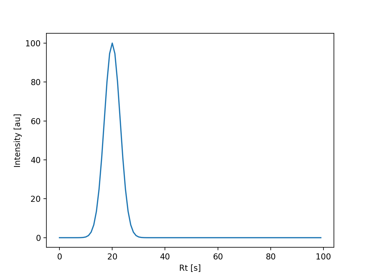
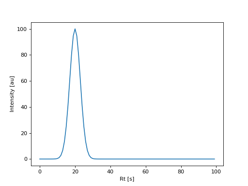
The following figure displays an extracted ion chromatogram created from this simulated sample:
(Source code, png, hires.png, pdf)
The SimulatedLCMSSampleFactory contains two fields:
- config
contains the parameters related with simulating the data acquisition conditions, such as time resolution, number of scans, m/z grid resolution, etc…
- adducts
contain a list adduct specifications, which define the features that will be observed in the data.
The sample factory configuration will be discussed in the Sample simulation section. We start by discussing the adduct specification in detail as it is the key component used in both sample and matrix data simulation.
Adduct specification#
The observed signal \(x\) is modelled using the following expression:
where \(f\) is the response factor, \(c\) is the abundance of the chemical species that generates the
adduct, \(p_{k}\) is the relative abundance of the corresponding isotopologue and \(\epsilon\) is an
additive noise term. Each one of these variables model different sources of variation observed in the data. The
SimulatedLCMSAdductSpec describes how each one of the terms in the equation
are computed.
The chemical characteristics are specified through the
formula and
n_isotopologues fields, which define the
chemical formula, and the number of isotopologues to simulate (one by default). The chemical formula is a
string representation of a sum formula and may include a charge as shown in the Chemical formulas
guide. Using these parameters the \(p_{k}\) is computed for each simulated isotopologue.
The AbundanceSpec model defines how the abundance \(c\) is computed
for a given sample. The mean abundance and variation is modeled as a gaussian distribution, allowing to emulate
variation between different observations. The prevalence field
allows to define the fraction of sample where the chemical species that generate the adduct will be observed.
By default a sample will have an abundance equal to 100, no variation between samples (\(\sigma=0\)) and
a prevalence equal to 1.
The response factor \(f\) can model time-dependent signal drift and inter-batch effects, but to keep the explanation as simple as possible the details about this are moved into the Computing the response factor section. If the default parameters are used, the response factor will be constant and equal to 1.
The additive noise \(\epsilon\) is computed using the MeasurementNoiseSpec,
which samples the noise from a Gaussian distribution, ensuring that the snr follows the following
relation:
where \(\textrm{SNR}\) is the SNR for the k-th isotopologue; \(\textrm{SNR}_{\textrm{base}}\) is the adduct base signal-to-noise ratio, and \(\textrm{SNR}_{\textrm{min}}\) is the minimum signal-to-noise ratio allowed. This allows to scale the snr of less abundant isotopologues. For this computation we define the snr as follows:
where \(\sigma\) is the standard deviation of the distribution that generates the noise. In the default configuration, the additive noise term is set to zero.
Finally, the chromatographic peak specification defines the properties of the chromatographic peak, such as
mean retention time, retention time variation across samples and chromatographic peak width. This specification
is defined by the tidyms2.simulation.lcms.RtSpec model. The observed retention time is sampled from
a gaussian using the mean retention time and the retention time dispersion. The peak shape is modelled using the
following expression:
where \(\textrm{Rt}\) is the observed retention time for a sample and \(w\) is the chromatographic peak width parameter. In the default configuration, peaks will have a retention time equal to 10 and a peak width equal to 3.
With this information, we can rewrite the adduct specification example to customize the appearance of the observed signals:
adducts_spec = [
    {
        "formula": "[C54H104O6]+",
        "n_isotopologues": 3,
        "abundance": {
            "mean": 500,
            "std": 50,
        },
        "rt": {
            "mean": 10.0,
            "std": 1.0,
            "width": 4.0,
        },
        "noise": {
            "snr": 200,
        }
    },
    {
        "formula": "[C27H40O2]+",
        "n_isotopologues": 2,
        "abundance": {
            "mean": 200,
            "std": 50,
            "prevalence": 0.7,
        },
        "rt": {"mean": 20.0},
    },
    {
        "formula": "[C24H26O12]+",
        "n_isotopologues": 5,
        "rt": {"mean": 30.0},
    },
]
Sample simulation#
We already covered the adduct specification, which defines the properties of features that are
observed in a sample. The other configuration available for the sample factory is the data
acquisition specification, defined by the DataAcquisitionSpec
model. This models allows to define:
instrumental noise (m/z and intensity)
time resolution
number of scans
data mode (profile or centroid)
Instrumental noise is an additive noise added to m/z and intensity values on each scan. The values
are samples from a gaussian distribution using the fields mz_std
and int_std respectively.
The number of scans and time resolution can be configured by the corresponding fields in the specification.
The min_int removes points in spectra with
intensities lower than this value. This parameter is particularly useful for data simulation in profile mode,
as it drastically reduces the size of simulated spectra.
In the default configuration, the data is simulated in centroid mode, without m/z or intensity noise, a time resolution equal to 1 and 100 scans.
The following example show simulated centroid data with a custom acquisition specification:
import matplotlib.pyplot as plt

from tidyms2.simulation.lcms import SimulatedLCMSSampleFactory
from tidyms2.io import MSData
from tidyms2.algorithms.raw import make_chromatograms, MakeChromatogramParameters

factory_spec = {
    "data_acquisition": {
        "n_scans": 100,
        "time_resolution": 0.5,
        "int_std": 2.0,
    },
    "adducts": [
        {
            "formula": "[C54H104O6]+",
            "n_isotopologues": 3,
            "abundance": {
                "mean": 500,
                "std": 50,
            },
            "rt": {
                "mean": 10.0,
                "std": 1.0,
                "width": 4.0,
            },
            "noise": {
                "snr": 200,
            }
        },
        {
            "formula": "[C27H40O2]+",
            "n_isotopologues": 2,
            "abundance": {
                "mean": 200,
                "std": 50,
                "prevalence": 0.7,
            },
            "rt": {"mean": 20.0},
        },
        {
            "formula": "[C24H26O12]+",
            "n_isotopologues": 5,
            "rt": {"mean": 30.0},
        },
    ],
}

simulated_sample_factory = SimulatedLCMSSampleFactory(**factory_spec)
sample = simulated_sample_factory(id="my_sample")
ms_data = MSData(sample)

mz = ms_data.get_spectrum(10).mz[0] # get the m/z value from the first feature


params = MakeChromatogramParameters(mz=[mz])
chrom = make_chromatograms(ms_data, params)[0]

fig, ax = plt.subplots()

ax.plot(chrom.time, chrom.int)
ax.set_xlabel("Rt [s]")
ax.set_ylabel("Intensity [au]")
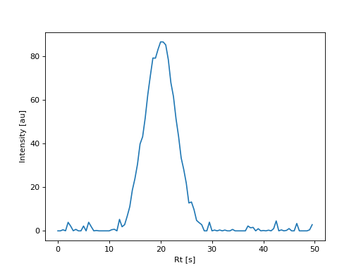
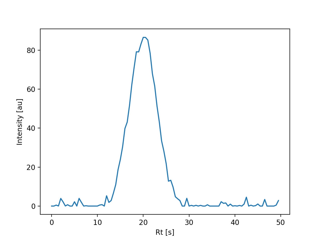
(Source code, png, hires.png, pdf)

EIC plot using simulated data with a custom acquisition specification.#
To simulate data in profile mode, an m/z grid specification must be provided. This specification is
defined by the MZGridSpec which defines the minimum and maximum
m/z values as well as the number of points in the grid. The generated grid is uniformly spaced, and
as MS data is sparse, it is useful to remove parts of the grid that do not contain useful information
using the min_int field. Finally, the
mz_width parameter controls the peak width
in the m/z dimension. This parameter allows to model signal overlap in the m/z domain, something that
cannot be done in centroid mode simulation. mz_width
is ignored in centroid mode.
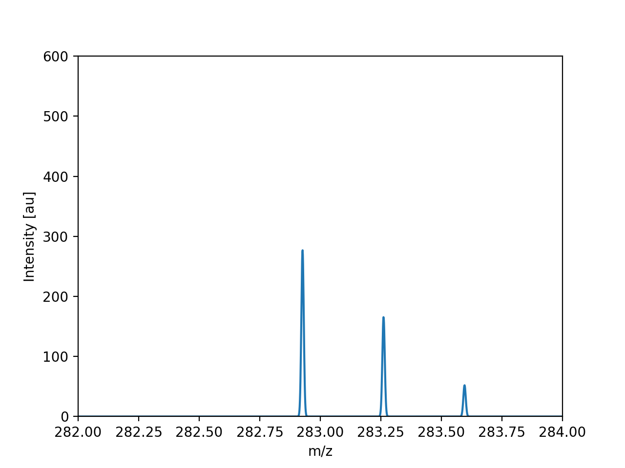
The following example show show an MS spectrum in profile mode:
(Source code, png, hires.png, pdf)
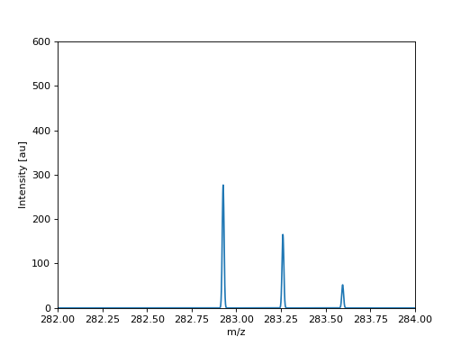
Simulated MS spectrum in profile mode.#
Data matrix simulation#
Data matrix simulation is a lot simpler to set up as no data acquisition specification is required. In this case, two things need to be defined:
an adduct specification
a list of samples to build the data matrix.
The following example shows a basic example of data matrix simulation:
from pathlib import Path

import matplotlib.pyplot as plt

from tidyms2.core.models import Sample
from tidyms2.simulation.lcms import SimulatedLCMSAdductSpec, simulate_data_matrix

formula_list = ["[C54H104O6]+", "[C27H40O2]+", "[C24H26O12]+"]
rt_list = [10.0, 20.0, 30.0]
abundances = [1000.0, 2000.0, 3000.0]
adducts = list()
for rt, abundance, formula in zip(rt_list, abundances, formula_list):
    adduct = SimulatedLCMSAdductSpec(
        formula=formula,
        n_isotopologues=2,
        abundance={"mean": abundance, "std": 20.0, "prevalence": 0.75},  # type: ignore
    )
    adducts.append(adduct)


samples = list()
for k in range(10):
    id_ = f"sample-{k}"
    path = Path.cwd() / f"{id_}.mzML"
    s = Sample(id=id_, path=path)
    s.meta.order = k
    samples.append(s)

data = simulate_data_matrix(adducts, samples)

col = data.get_columns(0)[0]
order = [s.meta.order for s in data.list_samples()]

fig, ax = plt.subplots()

ax.scatter(order, col.data)
ax.set_title(f"mz={col.feature.mz:.4f}, Rt={col.feature.descriptors["rt"]:.1f} s")
ax.set_xlabel("Run order")
ax.set_ylabel("Intensity [au]")
ax.set_ylim(0, 600.0)
(Source code, png, hires.png, pdf)

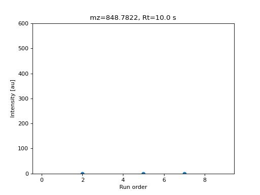
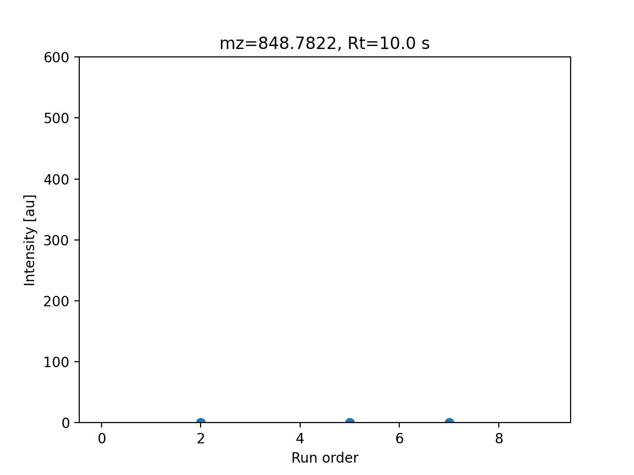
Data matrix value for a simulated feature.#
The Abundance specification can be defined on a per-group basis, by passing a dictionary that maps sample groups to abundance specifications. The following example defines two sample groups with different feature mean values:
(Source code, png, hires.png, pdf)
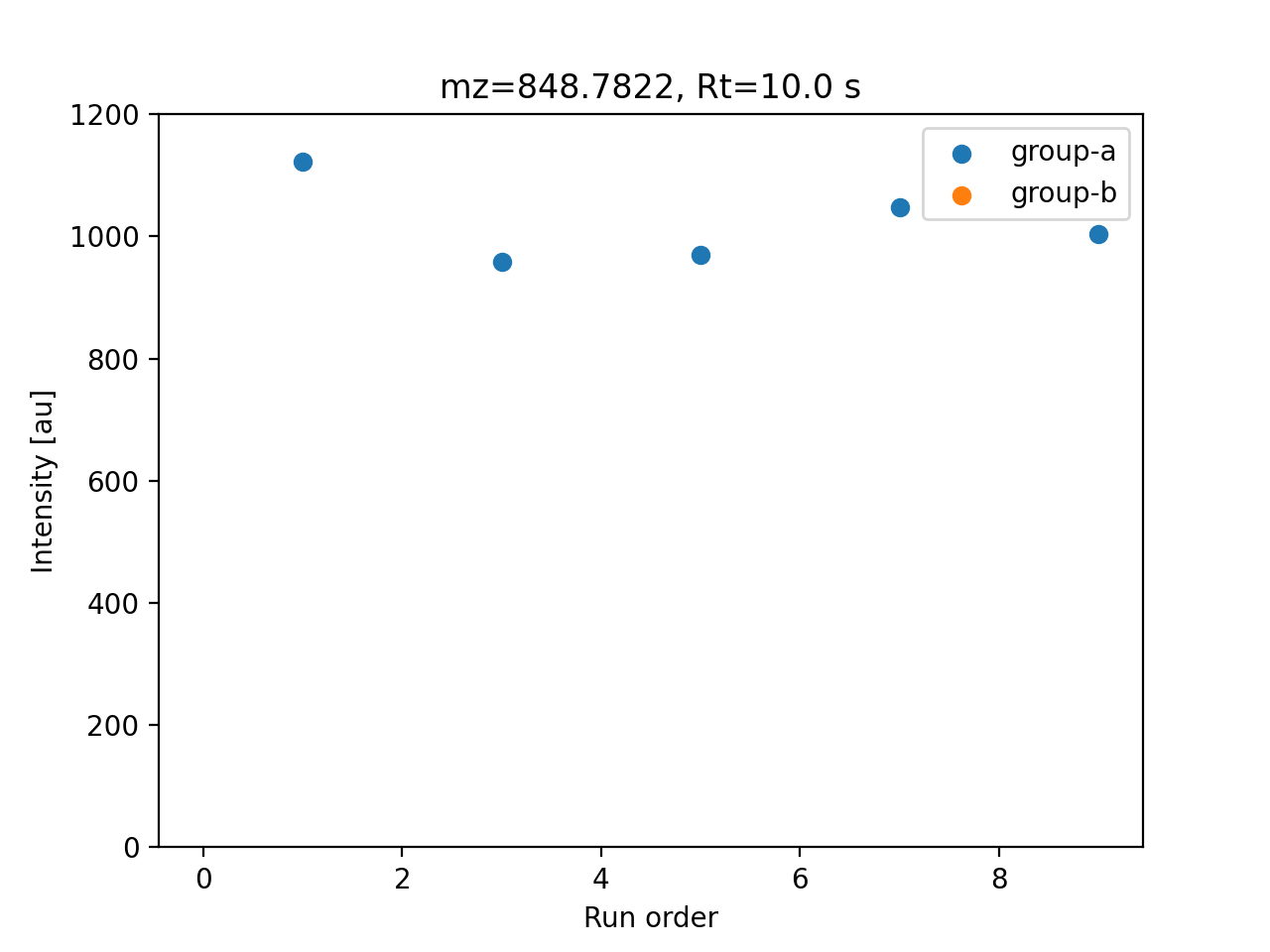
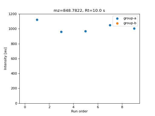
Data matrix value for a simulated feature.#
Computing the response factor#
The response factor \(f\) observed on each sample is defined by the
InstrumentResponseSpec model, which can be customized for each adduct.
In the default configuration no time-dependent effects are included. The response factor can be used to
model time-dependent variation between samples, as described by the following equation:
Where \(\tilde{f}\) is the base_response_factor,
\(M\) is the max_sensitivity_loss
and \(\lambda\) is the sensitivity_decay.
\(b\) is the inter-batch variation, a random value sampled from a uniform distribution
with minimum equal to the interbatch_variation
parameter and maximum equal to 1. This value is sampled once for each analytical batch value and applied
to all observations from that batch.
The following code example shows matrix data simulated with time-dependent effects:
(Source code, png, hires.png, pdf)
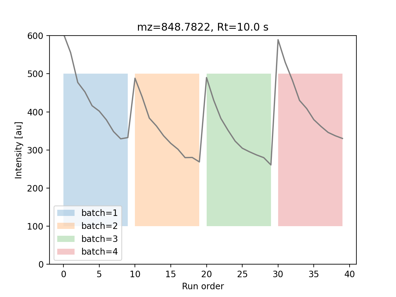
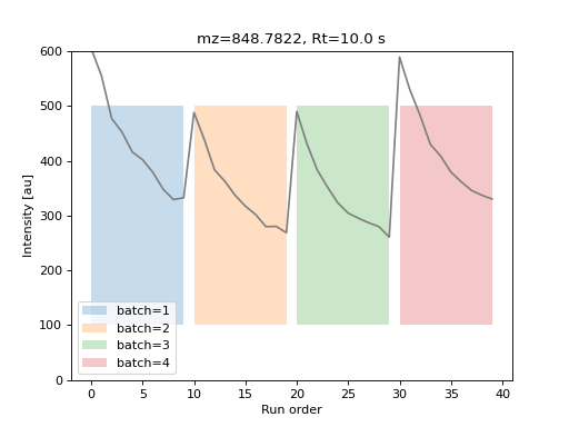
Data matrix value for a simulated feature with time-dependent variations.#